Conditional Formatting in Excel

This isn’t so much a cool “magical” tip as much as it’s a reminder to myself that it exists and I should use it more often. Excel has a Conditional Formatting feature that allows you to apply rules to a spreadsheet to have certain data situations display in different ways automatically.

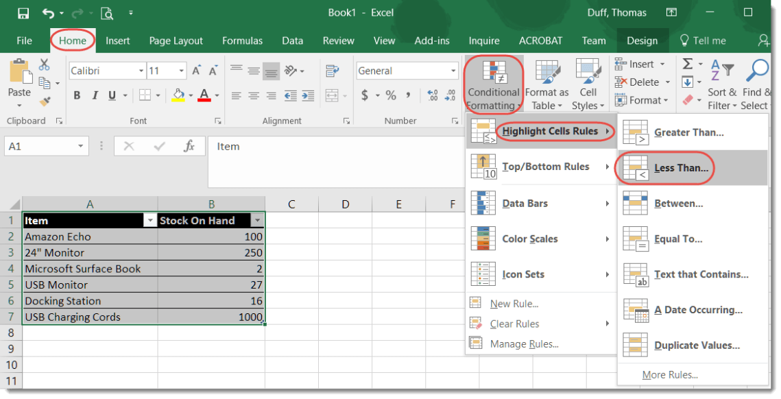
Here I have a spreadsheet with some items and numbers indicating the stock on hand for that item. I want to flag items that have less than 25 items so that I can reorder.  To set the conditional formatting, I select Home > Conditional Formatting > Highlight Cell Rules > Less Than…:

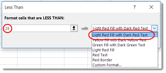
The Less Than dialog box appears, allowing me to specify a threshold total and how I want the cells to appear that meet that criteria:

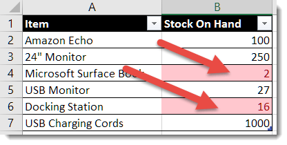
As soon as I save that, I now see the two items that need to be reordered as they dropped below 25 items:

This doesn’t even begin to scratch the surface of what you can do with conditional formatting, so go out there and play around some to see what you can do to make your data easier to read and to turn raw data into actionable information.